Built using Zelig version 5.1.4.90000

Least Squares Regression for Continuous Dependent Variables with ls.

Use least squares regression analysis to estimate the best linear predictor for the specified dependent variables.

Syntax

z.out <- zelig(Y ~ X1 + X2, model = "ls", weights = w, data = mydata)
x.out <- setx(z.out)
s.out <- sim(z.out, x = x.out)

For more details about the difference between Zelig’s reference classes and compatibility wrappers see the Quickstart Vignette.

The following examples typically use the compatibility wrappers.

Examples

Simple first differences

Load Zelig and attach example data frame:

library(Zelig)

## Loading required package: survival

data(macro)

Estimate model:

z.out1 <- zelig(unem ~ gdp + capmob + trade, model = "ls", data = macro,
                cite = FALSE)

Summarize regression coefficients:

summary(z.out1)

## Model: 
## 
## Call:
## z5$zelig(formula = unem ~ gdp + capmob + trade, data = macro)
## 
## Residuals:
##     Min      1Q  Median      3Q     Max 
## -5.3008 -2.0768 -0.3187  1.9789  7.7715 
## 
## Coefficients:
##              Estimate Std. Error t value Pr(>|t|)
## (Intercept)  6.181294   0.450572  13.719  < 2e-16
## gdp         -0.323601   0.062820  -5.151 4.36e-07
## capmob       1.421939   0.166443   8.543 4.22e-16
## trade        0.019854   0.005606   3.542 0.000452
## 
## Residual standard error: 2.746 on 346 degrees of freedom
## Multiple R-squared:  0.2878, Adjusted R-squared:  0.2817 
## F-statistic: 46.61 on 3 and 346 DF,  p-value: < 2.2e-16
## 
## Next step: Use 'setx' method

Set explanatory variables to their default (mean/mode) values, with high (80th percentile) and low (20th percentile) values for the trade variable:

x.high <- setx(z.out1, trade = quantile(macro$trade, 0.8))
x.low <- setx(z.out1, trade = quantile(macro$trade, 0.2))

Simulate first differences for the effect of high versus low trade on GDP:

s.out1 <- sim(z.out1, x = x.high, x1 = x.low)
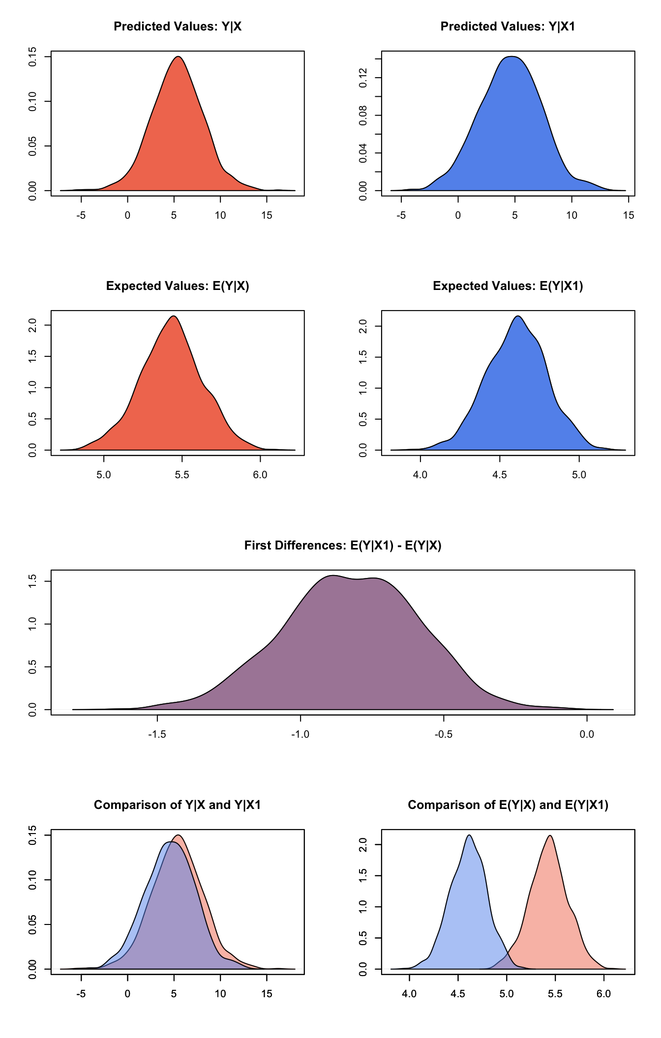
summary(s.out1)

## 
##  sim x :
##  -----
## ev
##       mean        sd      50%     2.5%    97.5%
## 1 5.430825 0.1975505 5.435411 5.032558 5.817717
## pv
##          mean       sd      50%       2.5%    97.5%
## [1,] 5.372131 2.780211 5.382567 0.04039063 11.09952
## 
##  sim x1 :
##  -----
## ev
##       mean        sd      50%     2.5%    97.5%
## 1 4.605703 0.1883663 4.609505 4.242307 4.971407
## pv
##          mean       sd      50%       2.5%    97.5%
## [1,] 4.581666 2.705597 4.624043 -0.8353483 9.890554
## fd
##         mean        sd        50%      2.5%      97.5%
## 1 -0.8251222 0.2384639 -0.8214742 -1.292467 -0.3886624

Plot the simulated distributions:

plot(s.out1)

Categorical variables, including fixed effects

Estimate a model with fixed effects for each country (see for help with dummy variables). Note that you do not need to create dummy variables, as the program will automatically parse the unique values in the selected variable into discrete levels.

z.out2 <- zelig(unem ~ gdp + trade + capmob + as.factor(country), model = "ls",
                data = macro, cite = FALSE)

Set values for the explanatory variables, using the default mean/mode values, with country set to the United States and Japan, respectively:

x.US <- setx(z.out2, country = "United States")
x.Japan <- setx(z.out2, country = "Japan")

Simulate quantities of interest:

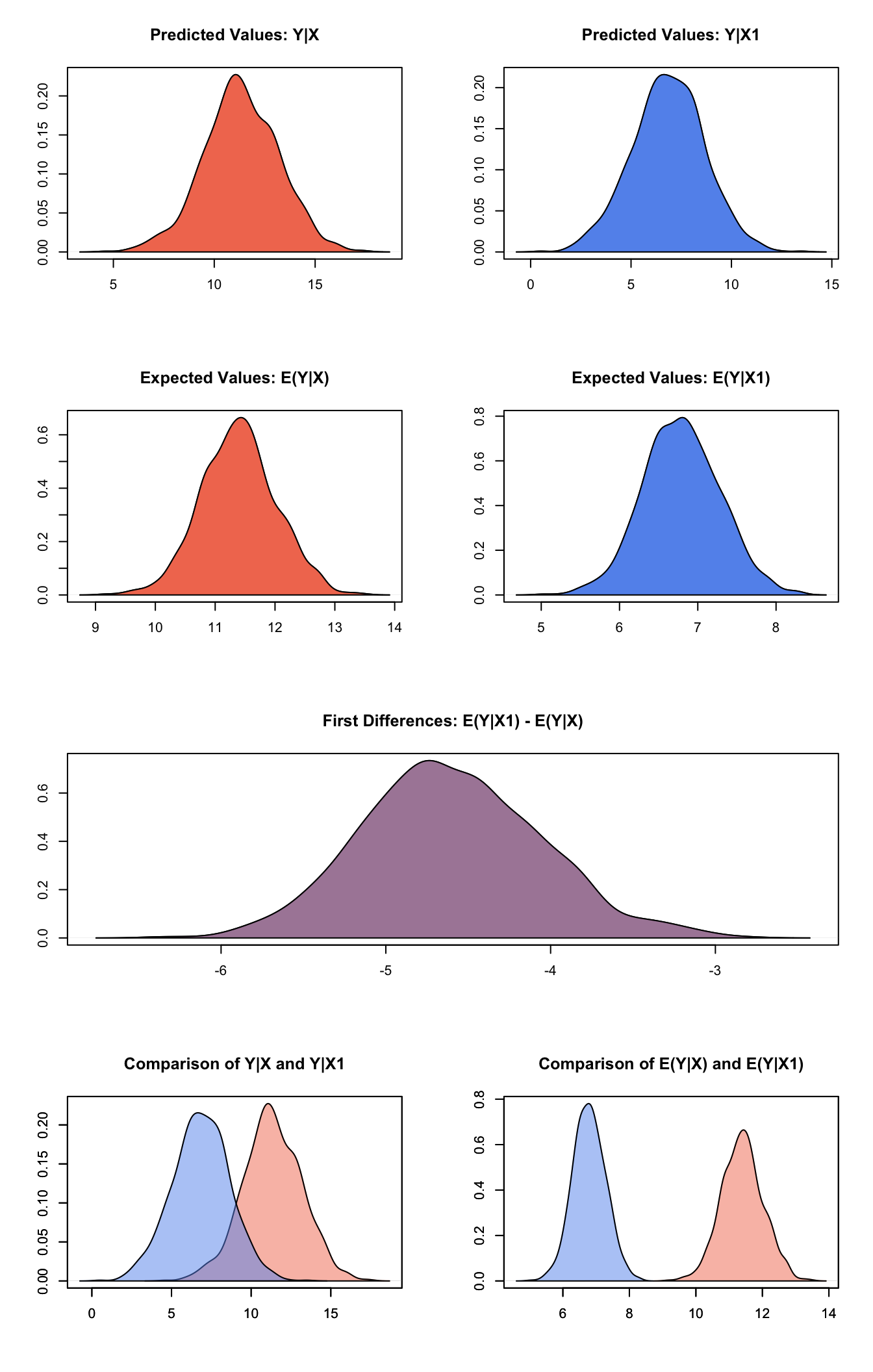
s.out2 <- sim(z.out2, x = x.US, x1 = x.Japan)

and plot the results:

plot(s.out2)

Model Definition

• The stochastic component is described by a density with mean \(\mu_i\) and the common variance \(\sigma^2\)

\[ Y_i \; \sim \; f(y_i \mid \mu_i, \sigma^2). \]

• The systematic component models the conditional mean as

\[ \mu_i = x_i \beta, \]

where \(x_i\) is the vector of covariates, and \(\beta\) is the vector of coefficients.

The least squares estimator is the best linear predictor of a dependent variable given \(x_i\), and minimizes the sum of squared residuals, \(\sum_{i=1}^n (Y_i-x_i \beta)^2\).

Quantities of Interest Definition

• The expected value (qi$ev) is the mean of simulations from the stochastic component,

\[ E(Y) = x_i \beta, \]

given a draw of \(\beta\) from its sampling distribution.

• In conditional prediction models, the average expected treatment effect (att.ev) for the treatment group is

\[ \frac{1}{\sum_{i=1}^n t_i}\sum_{i:t_i=1}^n \left\{ Y_i(t_i=1) - E[Y_i(t_i=0)] \right\}, \]

where \(t_i\) is a binary explanatory variable defining the treatment (\(t_i=1\)) and control (\(t_i=0\)) groups. Variation in the simulations are due to uncertainty in simulating \(E[Y_i(t_i=0)]\), the counterfactual expected value of \(Y_i\) for observations in the treatment group, under the assumption that everything stays the same except that the treatment indicator is switched to :math: \(t_i=0\).

Output Values

The output of each Zelig function call contains useful information which you may view. For example, using the z.out1 object we estimated above, then you may see the coefficients by using get_coef:

z.out1$get_coef()

## [[1]]
## (Intercept)         gdp      capmob       trade 
##  6.18129445 -0.32360059  1.42193926  0.01985421

or the variance-covariance matrix with get_vcov:

z.out1$get_vcov()

## [[1]]
##              (Intercept)           gdp       capmob         trade
## (Intercept)  0.203014830 -1.582154e-02 1.679720e-02 -2.014899e-03
## gdp         -0.015821542  3.946360e-03 1.721017e-03  7.907613e-05
## capmob       0.016797200  1.721017e-03 2.770329e-02  4.025728e-05
## trade       -0.002014899  7.907613e-05 4.025728e-05  3.142207e-05

For a default summary of information use either

z.out1$summarize()

## Model: 
## 
## Call:
## z5$zelig(formula = unem ~ gdp + capmob + trade, data = macro)
## 
## Residuals:
##     Min      1Q  Median      3Q     Max 
## -5.3008 -2.0768 -0.3187  1.9789  7.7715 
## 
## Coefficients:
##              Estimate Std. Error t value Pr(>|t|)
## (Intercept)  6.181294   0.450572  13.719  < 2e-16
## gdp         -0.323601   0.062820  -5.151 4.36e-07
## capmob       1.421939   0.166443   8.543 4.22e-16
## trade        0.019854   0.005606   3.542 0.000452
## 
## Residual standard error: 2.746 on 346 degrees of freedom
## Multiple R-squared:  0.2878, Adjusted R-squared:  0.2817 
## F-statistic: 46.61 on 3 and 346 DF,  p-value: < 2.2e-16
## 
## Next step: Use 'setx' method

or as we saw before using the wrapper, e.g. summary(z.out1).

• From the zelig() output object z.out, you may use the following ‘getter’ functions to extract:

• get_pvalue and get_se: p-values and standard errors, respectively.

• get_residuals: residuals.

• get_fitted: fitted values.

• get_df_residual: the residual degrees of freedom.

• get_model_data: the input data frame.

• You can extract the entire original fitted model object with from_zelig_model. For example:

ls.original <- from_zelig_model(z.out1)

You can then use summary and the component selector $ to extract:

• coefficients: the parameter estimates with their associated standard errors, \(p\)-values, and \(t\)-statistics.

  \[\hat{\beta} \; = \; \left(\sum_{i=1}^n x_i' x_i\right)^{-1} \sum x_i y_i\]

• sigma: the square root of the estimate variance of the random error \(e\):

  \[\hat{\sigma} \; = \; \frac{\sum (Y_i-x_i\hat{\beta})^2}{n-k}\]

• r.squared: the fraction of the variance explained by the model:

  \[R^2 \; = \; 1 - \frac{\sum (Y_i-x_i\hat{\beta})^2}{\sum (y_i - \bar{y})^2}\]

• adj.r.squared: the above \(R^2\) statistic, penalizing for an increased number of explanatory variables.

• cov.unscaled: a \(k \times k\) matrix of unscaled covariances.

For example:

ls.original <- from_zelig_model(z.out1)
summary(ls.original)$adj.r.squared

## [1] 0.2816635