Ordered Probit

Built using Zelig version 5.1.4.90000

Ordinal Probit Regression for Ordered Categorical Dependent Variables with oprobit in ZeligChoice.

Use the ordinal probit regression model if your dependent variables are ordered and categorical. They may take on either integer values or character strings. For a Bayesian implementation of this model, see .

Syntax

First load packages:

library(zeligverse)

z.out <- zelig(as.factor(Y) ~ X1 + X23,
               model = "oprobit", data = mydata)
x.out <- setx(z.out)
s.out <- sim(z.out, x = x.out, x1 = NULL)

If Y takes discrete integer values, the as.factor() function will order it automatically. If Y takes on values composed of character strings, such as “strongly agree”, “agree”, and “disagree”, as.factor()`` will order the values in the order in which they appear in Y. You will need to replace your dependent variable with a factored variable prior to estimating the model throughzelig()`. See below for more information on creating ordered factors.

Example

Creating An Ordered Dependent Variable

Load the sample data:

data(sanction)

Create an ordered dependent variable:

sanction$ncost <- factor(sanction$ncost, ordered = TRUE,
                         levels = c("net gain", "little effect", "modest lost", "major loss"))

Estimate the model:

z.out <- zelig(ncost ~ mil + coop, model = "oprobit", data = sanction)

## How to cite this model in Zelig:
##   William N. Venables, and Brian D. Ripley. 2011.
##   oprobit: Ordinal Probit Regression for Ordered Categorical Dependent Variables
##   in Christine Choirat, Christopher Gandrud, James Honaker, Kosuke Imai, Gary King, and Olivia Lau,
##   "Zelig: Everyone's Statistical Software," http://zeligproject.org/

Summarize estimated paramters:

summary(z.out)

## Model: 
## Call:
## z5$zelig(formula = ncost ~ mil + coop, data = sanction)
## 
## Coefficients:
##       Value Std. Error t value
## mil  0.2746     0.4660  0.5892
## coop 0.4938     0.1721  2.8699
## 
## Intercepts:
##                           Value  Std. Error t value
## net gain|little effect    0.6694 0.3090     2.1663 
## little effect|modest lost 2.7975 0.4764     5.8724 
## modest lost|major loss    2.7977 0.4764     5.8725 
## 
## Residual Deviance: 104.8956 
## AIC: 114.8956 
## (9 observations deleted due to missingness)
## Next step: Use 'setx' method

Set the explanatory variables to their observed values:

x.out <- setx(z.out)

Simulate fitted values given x.out and view the results:

s.out <- sim(z.out, x = x.out)
summary(s.out)

## 
##  sim x :
##  -----
## ev
##                       mean           sd          50%         2.5%
## net gain      4.222658e-01 6.115683e-02 4.192618e-01 3.059022e-01
## little effect 5.202798e-01 9.001411e-02 5.318661e-01 3.100651e-01
## modest lost   1.440359e-05 1.162046e-05 1.276885e-05 2.425079e-10
## major loss    5.743995e-02 7.666365e-02 2.460539e-02 7.625862e-08
##                      97.5%
## net gain      0.5469587564
## little effect 0.6607319292
## modest lost   0.0000355219
## major loss    0.2706138225
## pv
##       mean        sd 50% 2.5% 97.5%
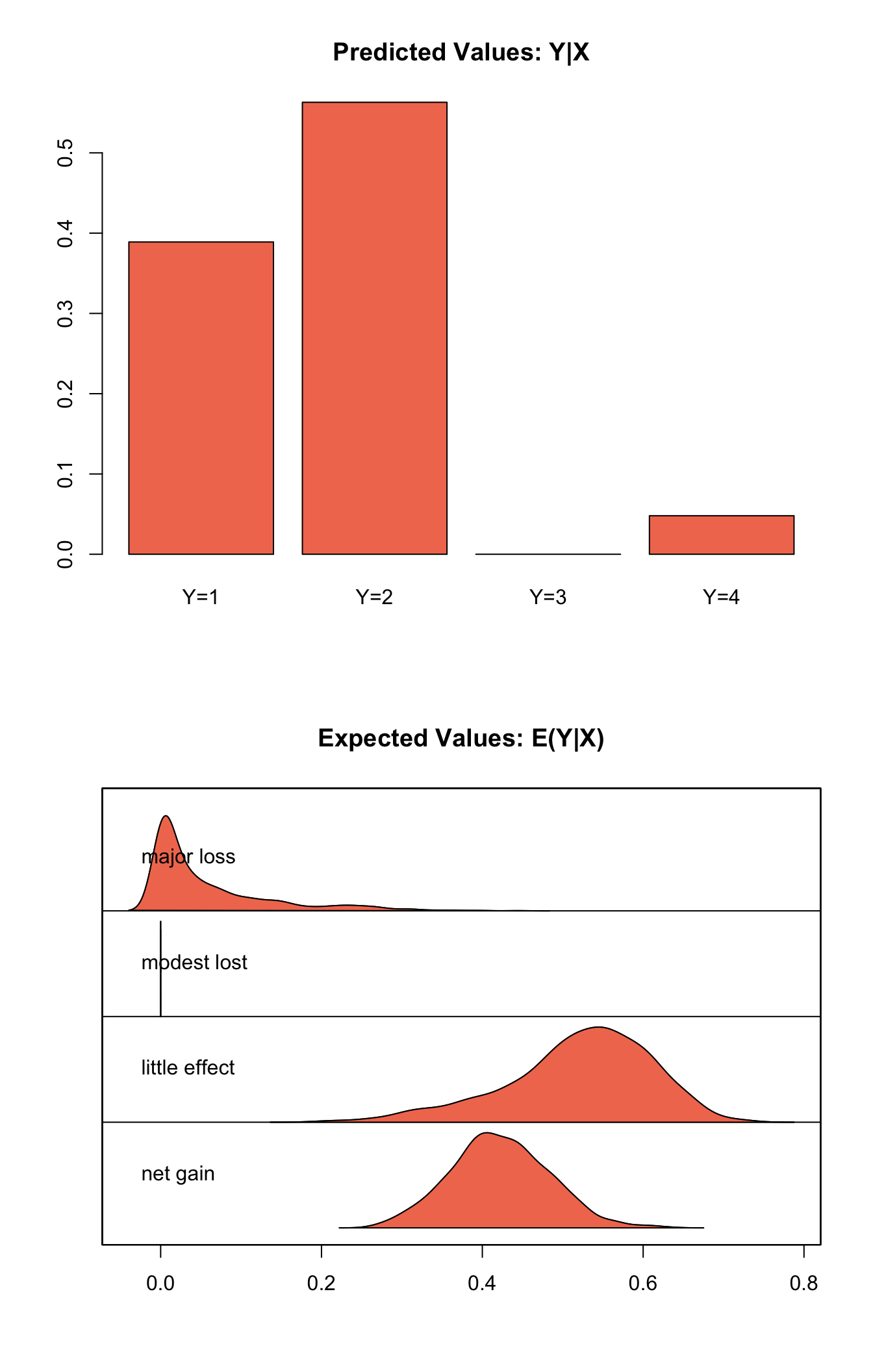
## [1,] 1.707 0.7040218   2    1     4

plot(s.out)

Graphs of Quantities of Interest for Ordered Probit

First Differences

Using the sample data sanction, let us estimate the empirical model and return the coefficients:

z.out <- zelig(as.factor(cost) ~ mil + coop, model = "oprobit",
               data = sanction)

## How to cite this model in Zelig:
##   William N. Venables, and Brian D. Ripley. 2011.
##   oprobit: Ordinal Probit Regression for Ordered Categorical Dependent Variables
##   in Christine Choirat, Christopher Gandrud, James Honaker, Kosuke Imai, Gary King, and Olivia Lau,
##   "Zelig: Everyone's Statistical Software," http://zeligproject.org/

summary(z.out)

## Model: 
## Call:
## z5$zelig(formula = as.factor(cost) ~ mil + coop, data = sanction)
## 
## Coefficients:
##         Value Std. Error  t value
## mil  -0.03531     0.4297 -0.08217
## coop  0.58713     0.1448  4.05584
## 
## Intercepts:
##     Value   Std. Error t value
## 1|2  0.6980  0.2801     2.4921
## 2|3  2.2498  0.3635     6.1900
## 3|4  3.1082  0.4399     7.0659
## 
## Residual Deviance: 153.536 
## AIC: 163.536 
## Next step: Use 'setx' method

Set the explanatory variables to their means, with coop set to 1 (the lowest value) in the baseline case and set to 4 (the highest value) in the alternative case:

x.low <- setx(z.out, coop = 1)
x.high <- setx(z.out, coop = 4)

Generate simulated fitted values and first differences, and view the results:

s.out2 <- sim(z.out, x = x.low, x1 = x.high)
summary(s.out2)

## 
##  sim x :
##  -----
## ev
##         mean         sd         50%         2.5%     97.5%
## 1 0.54063808 0.06781178 0.545177721 4.014215e-01 0.6686594
## 2 0.38773365 0.05351191 0.391120436 2.776921e-01 0.4893008
## 3 0.04890851 0.04001919 0.039261846 4.987695e-04 0.1359964
## 4 0.02271977 0.03986492 0.005083584 1.867483e-07 0.1418396
## pv
##       mean        sd 50% 2.5% 97.5%
## [1,] 1.599 0.7407751   1    1     4
## 
##  sim x1 :
##  -----
## ev
##         mean         sd        50%        2.5%     97.5%
## 1 0.05890804 0.04130743 0.05032893 0.009928432 0.1681794
## 2 0.43483566 0.16314387 0.41333016 0.187065246 0.8175809
## 3 0.27884079 0.08909879 0.27447653 0.121181259 0.4639010
## 4 0.22741551 0.16052194 0.20664215 0.003761621 0.5696715
## pv
##       mean        sd 50% 2.5% 97.5%
## [1,] 2.722 0.8874139   3    1     4
## fd
##          mean         sd         50%         2.5%      97.5%
## 1 -0.48173004 0.08367226 -0.48503281 -0.633651954 -0.3075439
## 2  0.04710202 0.15924106  0.01997809 -0.192669600  0.4199314
## 3  0.22993228 0.10335105  0.23147091  0.038869058  0.4254108
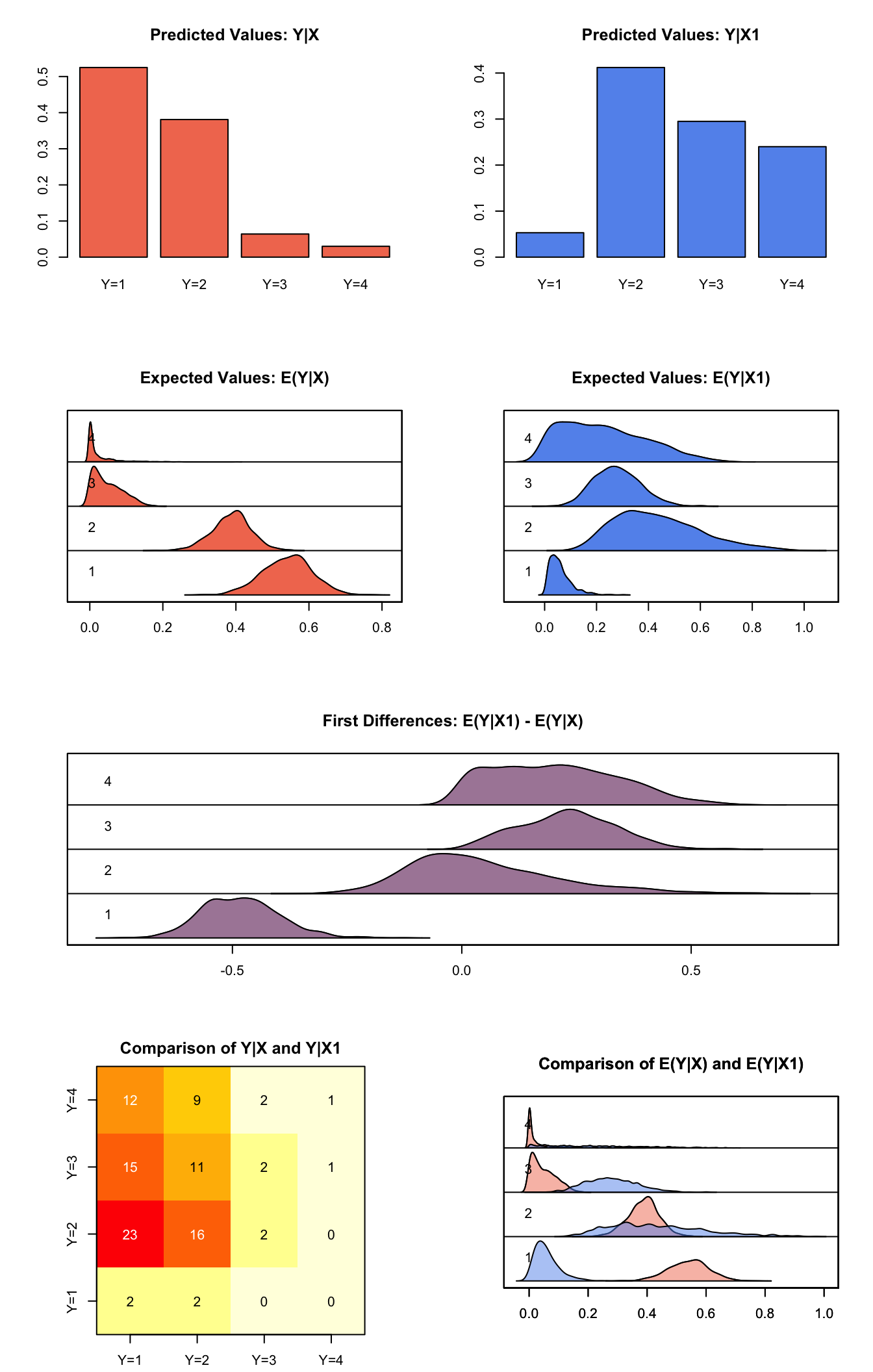
## 4  0.20469574 0.13486057  0.19740217  0.003761521  0.4765690

plot(s.out2)

Graphs of Quantities of Interest for Ordered Probit

Model

Let $Y_i$ be the ordered categorical dependent variable for observation $i$ that takes one of the integer values from $1$ to $J$ where $J$ is the total number of categories.

The stochastic component is described by an unobserved continuous variable, $Y^*_i$, which follows the normal distribution with mean $\mu_i$ and unit variance

\[ Y_i^* \; \sim \; N(\mu_i, 1). \]

The observation mechanism is

\[ Y_i \; = \; j \quad {\rm if} \quad \tau_{j-1} \le Y_i^* \le \tau_j \quad {\rm for} \quad j=1,\dots,J. \]

where $\tau_k$ for $k=0,\dots,J$ is the threshold parameter with the following constraints; [_l]( _m$ for all [l](m$ and $\tau_0=-\infty$ and $\tau_J=\infty$.

Given this observation mechanism, the probability for each category, is given by

\[ \Pr(Y_i = j) \; = \; \Phi(\tau_{j} \mid \mu_i) - \Phi(\tau_{j-1} \mid \mu_i) \quad {\rm for} \quad j=1,\dots,J \]

where $\Phi(\mu_i)$ is the cumulative distribution function for the Normal distribution with mean $\mu_i$ and unit variance.

The systematic component is given by

\[ \mu_i \; = \; x_i \beta \]

where $x_i$ is the vector of explanatory variables and $\beta$ is the vector of coefficients.

Quantities of Interest

The expected values (qi$ev) for the ordinal probit model are simulations of the predicted probabilities for each category:

\[ E(Y_i = j) \; = \; \Pr(Y_i = j) \; = \; \Phi(\tau_{j} \mid \mu_i) - \Phi(\tau_{j-1} \mid \mu_i) \quad {\rm for} \quad j=1,\dots,J, \]

given draws of $\beta$ from its posterior.

The predicted value (qi$pr) is the observed value of $Y_i$ given the underlying standard normal distribution described by $\mu_i$.
The difference in each of the predicted probabilities (qi$fd) is given by

\[ \Pr(Y=j \mid x_1) \;-\; \Pr(Y=j \mid x) \quad {\rm for} \quad j=1,\dots,J. \]

In conditional prediction models, the average expected treatment effect (qi$att.ev) for the treatment group in category $j$ is

\[ \begin{aligned} \frac{1}{n_j}\sum_{i:t_{i}=1}^{n_j}[Y_{i}(t_{i}=1)-E[Y_{i}(t_{i}=0)]],\end{aligned} \]

where $t_{i}$ is a binary explanatory variable defining the treatment ($t_{i}=1$) and control ($t_{i}=0$) groups, and $n_j$ is the number of treated observations in category $j$.

In conditional prediction models, the average predicted treatment effect (qi$att.pr) for the treatment group in category $j$ is

\[ \begin{aligned} \frac{1}{n_j}\sum_{i:t_{i}=1}^{n_j}[Y_{i}(t_{i}=1)-\widehat{Y_{i}(t_{i}=0)}],\end{aligned} \]

where $t_{i}$ is a binary explanatory variable defining the treatment ($t_{i}=1$) and control ($t_{i}=0$) groups, and $n_j$ is the number of treated observations in category $j$.

Output Values

The output of each Zelig command contains useful information which you may view. For example, if you run z.out <- zelig(y ~ x, model = oprobit, data), then you may examine the available information in z.out by using names(z.out), see the coefficients by using z.out$coefficients, and a default summary of information through summary(z.out). Other elements available through the $ operator are listed below.

From the zelig() output object z.out, you may extract:
coefficients: the named vector of coefficients.
fitted.values: an $n \times J$ matrix of the in-sample fitted values.
predictors: an $n \times (J-1)$ matrix of the linear predictors $x_i \beta_j$.
residuals: an $n \times (J-1)$ matrix of the residuals.
zeta: a vector containing the estimated class boundaries.
df.residual: the residual degrees of freedom.
df.total: the total degrees of freedom.
rss: the residual sum of squares.
y: an $n \times J$ matrix of the dependent variables.
zelig.data: the input data frame if save.data = TRUE.
From `summary(z.out)``, you may extract:
coef3: a table of the coefficients with their associated standard errors and $t$-statistics.
cov.unscaled: the variance-covariance matrix.
pearson.resid: an $n \times (m-1)$ matrix of the Pearson residuals.

2017-10-29